Numerical optimization is at the core of much of machine learning.
Gradient Descent
That’s not hard, we just jump to the conclusion.
To minimize the function \(f\), We update the value with \(x_{n+1}=x_n-γ∇f(x_n)\)
For python code, see here
Stochastic Gradient Descent and Mini-Batch Gradient Descent
The gradient descent algorithm may be infeasible when the training data size is huge. Thus, a stochastic version of the algorithm is often used instead. To motivate the use of stochastic optimization algorithms, note that when training deep learning models, we often consider the objective function as a sum of a finite number of functions:
\(f(x)=\frac{1}{n}∑_{i=1}^nf_i(x)\), where $f_i(x)$ is a loss function based on the training data instance indexed by i. When n is huge, the per-iteration computational cost of gradient descent is very high.
At each iteration a mini-batch $B$ (one single point if SGD) that consists of indices for training data instances may be sampled at uniform with replacement. Similarly, we can use
\[∇f_B(x)=\frac{1}{\lvert B\lvert}∑_{i∈B}∇f_i(x)\]to update x as
\[x_{n+1}=x_{n}−η∇f_B(x)\label{SGD}\]Momentum
SGD has trouble navigating ravines, i.e. areas where the surface curves much more steeply in one dimension than in another , which are common around local optima.

Momentum is a method that helps accelerate SGD in the relevant direction and dampens oscillations. It does this by adding a fraction \(μ\) of the update vector of the past time step to the current update vector:
\[v_{n+1}=μv_n-∇f(x_n)\\ x_{n+1}=x_n-γv_{n+1}\]We usually set $μ$ as 0.9 or similar value. From the formula we find that \(μ\) can accelerate speed at the very begining and reduce the change in oriention in ravines. Sometimes, it can jump out of the local minimum sine \(μ\) gives a great acceleration.
Nesterov accelerated gradient (NAG)
However, a ball that rolls down a hill, blindly following the slope, is highly unsatisfactory. We’d like to have a smarter ball, a ball that has a notion of where it is going so that it knows to slow down before the hill slopes up again.
Nesterov accelerated gradient (NAG) is a way to give our momentum term this kind of prescience. We know that we will use our momentum term \(γv_n\) to move the parameters \(x_n\). Computing $x_n−γv_n$ thus gives us an approximation of the next position of the parameters (the gradient is missing for the full update), a rough idea where our parameters are going to be. We can now effectively look ahead by calculating the gradient not w.r.t. to our current parameters \(x_n\) but w.r.t. the approximate future position of our parameters:
\[v_{n+1} = μv_n+∇f(x_n-γv_n)\\ x_{n+1}=x_n-γv_{n+1}\]Again, we set the momentum term γ to a value of around 0.9. While Momentum first computes the current gradient (small blue vector in Image 4) and then takes a big jump in the direction of the updated accumulated gradient (big blue vector), NAG first makes a big jump in the direction of the previous accumulated gradient (brown vector), measures the gradient and then makes a correction (red vector), which results in the complete NAG update (green vector). This anticipatory update prevents us from going too fast and results in increased responsiveness, which has significantly increased the performance of RNNs on a number of tasks.

See Convolutional Neural Networks for another ituitive explanation of NAG.
Adagrad
In machine learning, we should not always set learning rating manually. Usually we use Adaptive learning rate. Here we introduce adagrad. Adagrad is the extension Gradient Descent with L2 regularizer on gradient.
\[g_n=∇f(x_n)\\ G_n=diag(g_n^2)+G_{n-1}\\ ϵ<<0\\ x_{n+1} = x_n-\frac{γ}{\sqrt{ϵ+G_n}}g_n\]With adagrad, now we will converge more quickly.

Adadelta
Adadelta is an extension of Adagrad that seeks to reduce its aggressive, monotonically decreasing learning rate. Instead of accumulating all past squared gradients, Adadelta restricts the window of accumulated past gradients to some fixed size \(ω\).
\[E[g^2]_n=ωE[g^2]_{n-1}+(1-ω)g^2_n\\ x_{n+1}=x_n-\frac{γ}{\sqrt{ϵ+E[g^2]_n}}g_n\]where \(E[g^2]\) doesnot mean the expectation of \(g^2\), but the running average value. (Such notation of \(E(f(y))_n=ωE(f(y))_{n-1}+(1-ω)f(y_n)\))
The denominator is just the root mean squared error (RMS) critrerion of the gradient, i.e. \(RMS[g]_n=\sqrt{ϵ+E[g^2]_n}\)
According to Matthew D. Zeiler “An Adaptive Learning Rate Method” note that the units in this update (as well as in SGD, Momentum, or Adagrad) do not match, i.e. the update should have the same hypothetical units as the parameter.
The first order methods: units of \(Δx∝\) units of \(g∝∇f∝\) units of \(\frac{1}{x}\)
The second order methods: units of \(H^{-1}g∝\frac{∇f}{∇^2f}∝\) units of x
To realize this, they first define another exponentially decaying average. It’s similar to the \(E[g^2]_n\). this time not of squared gradients but of squared parameter updates:
\[E[Δx^2]_n=γE[Δx^2]_{n-1}+(1-γ)Δx^2_n\]Then notice that:
\[∆x = \frac{g}{H}\\ \frac{1}{H}=\frac{Δx}{g}\]We can now apply the Newton’s Method on it. Since the RMS of the previous gradients is already represented in the denomitator, we consider a measure of the \(Δx\) quantity in the numerator. That is \(RMS[Δx]_{n}\). Because we donot know\(Δx\), we replace it with \(Δx_{n-1}\). Our final model is:
\[Δx_n=-\frac{RMS[Δx]_{n-1}}{RMS[g]_n}g_n\\ x_{n+1}=x_n+Δx_n\]RMSprop
RMSprop is an unpublished, adaptive learning rate method proposed by Geoff Hinton in Lecture 6e of his Coursera Class. It is a special case of AdaDelta.
\[Δx_n=-\frac{\gamma}{RMS[g]_n}g_t\]Adaptive Moment Estimation (Adam)
Adaptive Moment Estimation is another method that computes adaptive learning rates for each parameter. It add exponentially decaying average on both first and second order momentum.
\[m_n=β_1m_{n-1}+(1-β_1)g_n\\ v_n=β_2v_{n-1}+(1-β_2)g_n^2\]Then we find that \(E[m_n]=E[g_n]\), and \(E[v_n] = E[g_n^2]\), that is the unbiased estimators of the first and second order of \(g\). But it will not hold in moving average!
\[m_n=(1-β_1)∑_{i=0}^nβ_1^{n-i}g_i\\ E[m_n]=E[g_i](1-\beta_1^n)+ξ\]So we need the correction:
\[\hat{m}_n=\frac{m_n}{1-\beta_1^n}\\ \hat{v}_n=\frac{v_n}{1-β_2^n}\]And finally is the update model:
\[x_{n+1}=x{n}-\frac{γ}{\sqrt{\hat{v_n}+ϵ}}\hat{m}_n\]AdaMax
The \(v_t\) factor in the Adam update rule scales the gradient inversely proportinally to the \(l_2\) norm of past gradients and current gradients. But we can extend it to \(l_p\) norm.
\(v_n=β_2^pv_{n-1}+(1-β_2^p)\lvert g_n\rvert ^p\) If we let \(p→∞\),
\[u_n=max(\beta_2v_{n-1},\lvert g_n\rvert)\] \[Δx_n=-\frac{γ}{u_n}\hat{m}_n\]When gradient comes to zero, it is more robust to the gradient noise.
Nesterov-accelerated Adaptive Moment Estimation (Nadam)
As we have seen before, Adam can be viewed as a combination of RMSprop and momentum: RMSprop contributes the exponentially decaying average of past squared gradients \(v_t\), while momentum accounts for the exponentially decaying average of past gradients \(m_t\). We have also seen that Nesterov accelerated gradient (NAG) is superior to vanilla momentum.
to be continued…
Newton’s Method
Suppose we want to reach the global minimizer of $f$ with parameter x. Suppose, we have an estimate $x_n$ and we wangt out next estimate $x_{n+1}$ to have the property that $f(x_{n+1})\lt f(x_n)$. Newton’s method use the taylor expansion:
\[f(x+Δx)≈f(x)+Δx^T∇f(x)+\frac{1}{2}Δx^T(∇^2f(x))Δx\], where $∇f(x)$ and $∇^2f(x)$ are the gradient and Hessian of f at the point $x_n$. This approximation holds when $‖Δx‖→0$.
Without loss of generality, we can write $x_{n+1}=x_n+Δx$ and re-write the above equation,
\[f(x_{n+1})≈h_n(Δx)=f(x_n)+Δx^Tg_n+\frac{1}{2}Δx^TH_nΔx\],where $g_n$ and $H_n$ represent the gradient and Hessian of $f$ at $x_n$.
If we take the differentiation with respect to $Δx$ and set it to zero yields: \(Δx=−H^{−1}_ng_n\) That is to say: \(x_{n+1}=x_n−α(H^{−1}_ng_n)\)
Quasi-Newton
The central issue with NewtonRaphson is that we need to be able to compute the inverse Hessian matrix. Usually, it’s computational large. Thus we introduce Quasi-Newton. The Quasi-Newton can update \(H^{-1}_n\) according to \(H^{-1}_{n-1}\)
Secant Condition
From taylor expansion we have \(f(x_{n+1})≈h_n(Δx)=f(x_n)+Δx^Tg_n+\frac{1}{2}Δx^TH_nΔx\), and let’s think about what’s the good property for $h_n(Δx)$.
Actually, we’d like to ensure $h_n()$ have the same first order derivation as $f()$ at point $x_n$ and $x_{n-1}$: \(∇h_n(x_n)=g_n\), and \(∇h_n(x_{n−1})=g_{n-1}\) We combine these two conditions together: \(∇h_n(x_n)−∇h_n(x_{n−1})=g_n−g_{n−1}\)
Use the derivation of formula (\ref{SGD}), we have:
\((x_n−x_{n−1})H_n=(g_n−g_{n−1})\) This is the so-called “secant condition” which ensures that $H_{n-1}$ behaves like the Hessian at least for the difference \(x_n-x_{n-1}\). Assuming \(H_n\) is invertible, then multiplying both sides by \(H_n^{-1}\) yields:
\[(x_n−x_{n−1})=(g_n−g_{n−1})H_n^{-1}\]or
\[s_n=y_nH^{-1}_n\label{secant}\]According to fomula (\ref{secant}), we can calculate the inverse Hessian matrix with only \(s_n\) and \(y_n\).
BFGS Update
Intuitively, we want Hn to satisfy the two conditions above:
- Secant condition holds for $s_n$ and $y_n$
- \(H_n\) is symmetric
Given the two conditions above, we’d like to take the most conservative change relative to \(H_{n−1}\). This is reminiscent of the MIRA update, where we have conditions on any good solution but all other things equal, want the ‘smallest’ change.
\[min_{H^{-1}}‖H^{-1}-H^{-1}_{n-1}‖^2\\ s.t.\ H^{-1}y_n=s_n\\ \ \ \ \ \ \ \ H^{-1}\ is\ symmetric\], The norm used here ∥⋅∥ is the weighted frobenius norm. The solution is given by
\[H^{−1}_{n+1}=(I−ρ_ny_ns^T_n)H^{−1}_n(I−ρ_ns_ny^T_n)+ρ_ns_ns^T_n\],where \(ρ_n=(y^T_ns_n)^{−1}\). The proof out the solution is outside of scope of this post. And for BFGS, we can use any initial matrix \(H_0\) as long as it is positive definite and symmetric.
Visualization
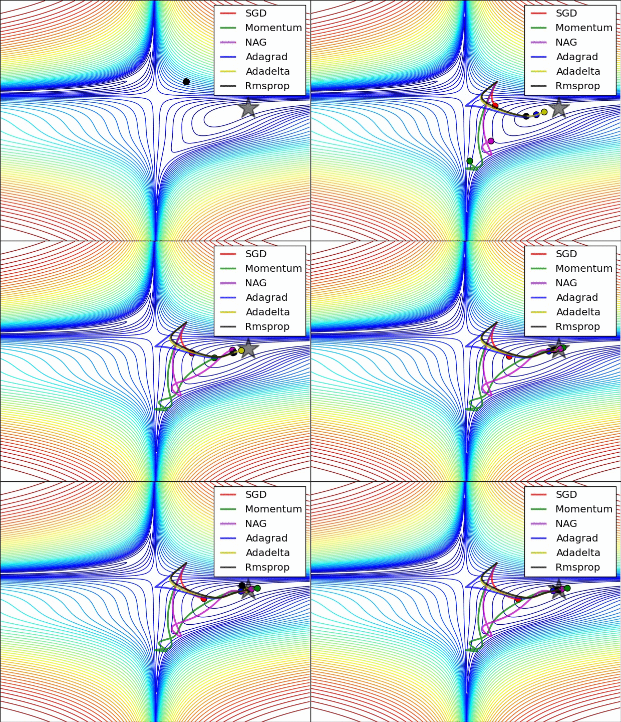
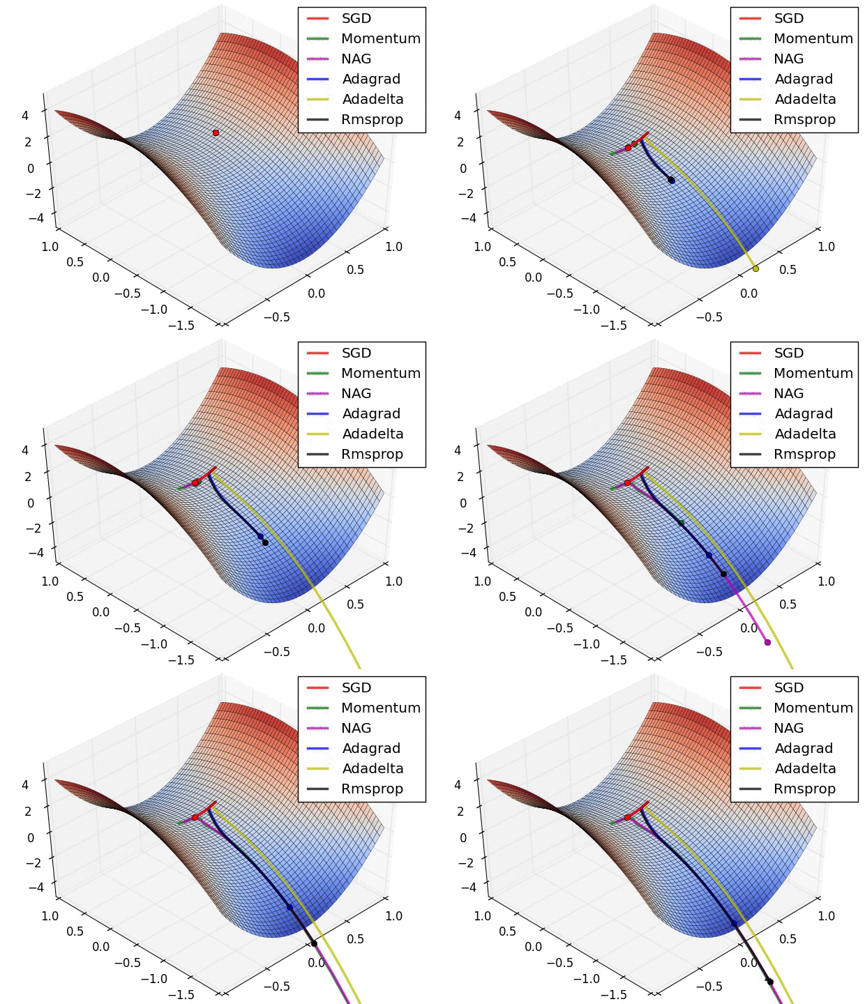
The following two animations (Image credit: Alec Radford) provide some intuitions towards the optimization behaviour of most of the presented optimization methods.


Summary
Momentum
Beginning: Quick Ending: oscillating in minimum with opposite direction May git rid of local minimum. Avoid ravines.
NAG
Similar to Momentum, but the correction avoid decresing too quickly
Adagrad
Beginning: Gradient Boosting Ending: Gradient shrinkage, early stop Can solve Gradient Vanish/Exploding, I will write some related topics later.(later)[https://medium.com/learn-love-ai/the-curious-case-of-the-vanishing-exploding-gradient-bf58ec6822eb] Suitable for (sparse gradient)[?????]. It will rely on hyperparameter.
AdaDelta
Beginning: Quick Ending: oscillating around local (global) minimum In the end will not git rid of local minimum, but you can switch to the momentum SGD to jump out the local minimum. If you switch back to AdaDelta later, it is still stuck in another local minimum. So the total accuracy may not change if you combine AdaDelta and momentum SGD. It also tells us why the simple SGD is still in the state of art. Use adaptive learning rate.
RMSprop
Good at unstable optimization function like RNN.(Need to learn)[??????] Still need hyperparameter.
Adam
Combine Momentum SGD (handle unstable optimization) and Adagrad (handle sparse gradient). Need less memory. Can handel non-convex problem and high dimension data.
AdaMax
Handle sparse parameter updates like word embeddings.
Reference
- GLUON Gradient descent and stochastic gradient descent from scratch
- Aria Numerical Optimization: Understanding L-BFGS